Live visualisation

Route optimisation is a spatial problem, and a solver's progress is easiest to judge by eye: are the crossings disappearing, is the best tour still changing, did the annealer freeze too early? skroute.viz draws the answer — a fitted solution as a static picture, a running solver live, and a finished run again, at time-lapse speed — through the fit(..., callback=) protocol every solver implements: the solver hands a RouteEvent to your callback at the start of the search, after every outer iteration (or every construction step) and at the end; LivePlot redraws the attempt, the best tour and the structure being built on each event, Recorder keeps them, with their clock, for later.

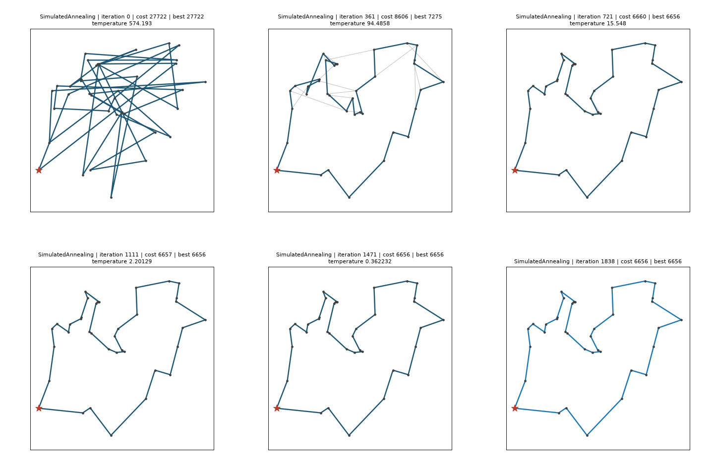
The pictures on this page are produced by the code of the repository: examples/live_demo.py --record writes them (the exact commands are given under each).

Installing

The package is optional and nothing else in scikit-route imports it:

pip install "scikit-route[viz]"       # matplotlib: plot_route, plot_history, LivePlot, Recorder
pip install "scikit-route[viz-map]"   # + plotly: OpenStreetMap tiles, the plotly backend, sliders

import skroute.viz needs neither library — matplotlib and plotly are loaded at the first call — and a missing one raises an ImportError naming the extra to install.

Coordinates are always (n, 2) arrays in the row order of the cost matrix. The matplotlib tools draw column 0 as x and column 1 as y; the map tools expect (latitude, longitude). For geographic data on plain axes pass coords[:, ::-1].

A picture of a solution

plot_route takes a fitted estimator and draws the nodes, the depot (a star) and the closed route, one colour per trip; the coordinates come from fit(..., coords=) or from its coords= argument. plot_history draws history_, the best-so-far cost per outer iteration.

>>> import matplotlib
>>> matplotlib.use("Agg")  # this page runs headless; drop the line on a desktop
>>> from skroute import IteratedLocalSearch
>>> from skroute.datasets import load_tsp
>>> from skroute.viz import plot_history, plot_route
>>> dj = load_tsp("dj38")  # Djibouti, 38 cities, optimum 6656
>>> ils = IteratedLocalSearch(random_state=0).fit(dj.distance_matrix(), labels=dj.labels, coords=dj.coords)
>>> ax = plot_route(ils)
>>> len(ax.lines), len(ax.lines[0].get_xdata())  # one closed trip through the 38 cities
(1, 39)
>>> ax.get_title().startswith("IteratedLocalSearch | cost ")
True
>>> ax = plot_history(ils)
>>> len(ax.lines[0].get_ydata()) == ils.n_iter_
True

A multi-trip solution gets one line per trip. plot_route also accepts a route array whose entries index the rows of coords (the tour_ or route_ of a solver fitted without labels=; a repeated depot separates trips) and any RouteEvent:

>>> import numpy as np
>>> xy = np.array([[0.0, 0.0], [1.0, 0.0], [1.0, 1.0], [0.0, 1.0]])
>>> ax = plot_route([0, 1, 0, 2, 3], xy, labels=True)  # two trips: 0-1-0 and 0-2-3-0
>>> len(ax.lines), [t.get_text() for t in ax.texts]
(2, ['0', '1', '2', '3'])

Watch a run live

LivePlot is a callable: pass it as the callback of fit. On the "start" event it opens the figure; on every every-th "iteration" event it redraws the current tour — the attempt the solver is working on — as a thin light line and the best tour so far as a thick one, and puts the solver, the iteration, both costs and one fact of the solver's own — its most informative scalar: the temperature of an annealer, the tenure of a tabu search... — in the title; on "end" it draws the final route with trip colours. It refreshes the window with plt.pause, so it never blocks and never calls plt.show() — add that yourself after fit to keep the window open.

>>> import matplotlib.pyplot as plt
>>> from skroute import SimulatedAnnealing
>>> from skroute.viz import LivePlot
>>> live = LivePlot(dj.coords, every=10)  # redraw every tenth temperature level
>>> sa = SimulatedAnnealing(random_state=0).fit(
...     dj.distance_matrix(), labels=dj.labels, callback=live
... )  # doctest: +SKIP
>>> plt.show()  # doctest: +SKIP

show= picks what to draw during the run — "both" (the default), "best" alone, or "current" alone — and trail=k keeps the last k attempts on screen, fading with age, which gives a sense of where the search has been:

>>> attempts = LivePlot(dj.coords, every=5, show="current", trail=8)  # the walker and its eight last steps
>>> attempts.show, attempts.trail
('current', 8)

A redraw costs a few milliseconds and a fast solver emits thousands of outer iterations per second, so every= is the knob that keeps the search fast: SimulatedAnnealing runs about 1 800 levels, IteratedLocalSearch up to n_iter kicks, TabuSearch n_iter moves. Headless machines work too — on the Agg backend the lines are updated on every kept iteration and the picture is rendered once, at "end", without being shown, which is how this page and the test-suite run.

The figure stays open after fit (close it with plt.close(live.fig) when you watch many runs in one script), and the same LivePlot can watch the next fit: a new "start" opens a fresh figure. Under MultiStart(..., n_jobs=1) the inner solvers' events are forwarded, so every restart is drawn from scratch in the same figure and its final route stays on screen until the next restart begins.

examples/live_demo.py in the repository wraps this in a small command line:

python examples/live_demo.py --instance dj38 --solver IteratedLocalSearch
python examples/live_demo.py --instance barcelona --solver SimulatedAnnealing --every 10 --show current --trail 5

In a notebook

The same object works in Jupyter. LivePlot detects the kernel and picks the refresh that fits the matplotlib backend:

• %matplotlib inline (the default) — every redraw replaces the cell output through IPython.display.display(fig, clear=True), and the figure is closed after the last one, so the cell ends with a single picture; keep every= generous, each redraw renders a PNG.
• %matplotlib widget (ipympl) — the canvas is updated in place, the way a desktop window is.
• LivePlot(coords, backend="plotly") — a Plotly FigureWidget displayed once and updated in place; map=True puts it on OpenStreetMap tiles (and selects this backend by itself). Needs scikit-route[viz-map] and anywidget (Plotly's widget dependency); without a kernel the plotly backend builds a plain Figure and shows it once at "end".

>>> live = LivePlot(dj.coords, backend="plotly", every=5)  # doctest: +SKIP
>>> IteratedLocalSearch(random_state=0).fit(dj.distance_matrix(), labels=dj.labels, callback=live)  # doctest: +SKIP

Replay at time-lapse speed

Recorder draws nothing while the solver runs; it copies every event (every= thins the iterations) together with the wall clock at which it arrived, and replays the run afterwards — as fast or as slow as you like. The deterministic descent below has three events; a real run has hundreds:

>>> from skroute import TwoOpt
>>> from skroute.viz import Recorder
>>> C = np.array([[0, 5, 9, 10], [5, 0, 4, 8], [9, 4, 0, 3], [10, 8, 3, 0]], dtype=float)
>>> rec = Recorder()
>>> two = TwoOpt().fit(C, coords=xy, callback=rec)
>>> [e.stage for e in rec.events], rec.n_frames
(['start', 'iteration', 'end'], 3)
>>> bool(np.all(np.diff(rec.timestamps) >= 0))  # the recorded clock, in seconds
True

Four ways to play it back:

• replay drives a LivePlot through the recorded events on the recorded clock divided by speed: rec.replay(coords, speed=10) shows a 30-second run in three seconds, in a window or a notebook, as it looked live — the time a redraw takes is absorbed by the waits that follow, a gap over two seconds is cut down to two, and where nothing is shown before "end" (the Agg backend) the events are drawn back to back. It returns the LivePlot (so live.fig holds the final picture); every=, show=, trail= and the other LivePlot options pass through.
• animate builds the same frames as a matplotlib FuncAnimation: plt.show() plays it, IPython.display.HTML(anim.to_jshtml()) embeds it in a notebook. With speed= (the default, 1.0, is real time) every frame waits its recorded gap divided by speed, clipped to [10, 2000] ms so a burst of iterations never flashes past and a slow step never freezes the replay (the floor is per frame: a run denser than a hundred kept frames per replayed second stretches rather than speeds up — thin it with Recorder(every=)); fps= plays one frame per kept event at a fixed rate instead; interval= fixes the delay in milliseconds; hold= is the pause on the final picture before the loop restarts. rec.frame_delays(speed=...) returns the per-frame delays in milliseconds.
• save writes the animation: a .gif through pillow, an .mp4 (or any format ffmpeg writes) through matplotlib's ffmpeg writer — a clear RuntimeError names ffmpeg when it is missing. fps= is the frame rate of the file; speed= turns it into a time-lapse (each frame is held for its recorded gap divided by speed, clipped to [10, 2000] ms like frame_delays and rounded to whole frames; a GIF folds repeated frames, so the time-lapse costs no extra bytes); the coordinates default to those of the fit.
• to_plotly gives a figure with one frame per kept event, Play/Pause buttons, a speed menu — 0.5x, 1x, 2x, 4x and 8x of fps — and a slider over the iterations; map=True puts it on OpenStreetMap tiles.

>>> live = rec.replay(xy, speed=1e9)  # no waiting at that speed: the three events, drawn in turn
>>> live.n_events, len(live.ax.lines) - 4  # after the four fixed artists: the final route, one trip
(3, 1)
>>> rec.frame_delays(speed=1e9).tolist()  # microsecond gaps at 1e9x: clipped to the 10 ms floor
[10.0, 10.0, 10.0]
>>> anim = rec.animate(xy, speed=10)  # doctest: +SKIP
>>> plt.show()  # doctest: +SKIP
>>> rec.save("descent.gif", xy, fps=20, speed=10)  # a 10x time-lapse GIF  # doctest: +SKIP
>>> rec.save("descent.mp4", xy, fps=30)  # ffmpeg on the PATH  # doctest: +SKIP
>>> fig = rec.to_plotly(xy)
>>> [b.label for b in fig.layout.updatemenus[1].buttons]
['0.5x', '1x', '2x', '4x', '8x']
>>> len(fig.frames) == rec.n_frames and [b.label for b in fig.layout.updatemenus[0].buttons]
['Play', 'Pause']
>>> fig.write_html("descent.html")  # doctest: +SKIP

Every frame is drawn the way LivePlot draws a live event — the attempt thin, the best tour thick, the structures of the next two sections when the solver reports them, the status line as the title, the final route with trip colours at "end" — and show= chooses the tours ("both", "best", "current") in replay, animate, save and to_plotly alike.

rec.events holds the copies (stage, iteration, cost, best_cost, tour, best_tour, extra, timestamp, a reference to the problem, and the decoded route and trips like a live event); rec.costs, rec.best_costs, rec.iterations and rec.timestamps are the same facts as arrays. A frame is drawn for every kept event that carries something to draw — a tour, a best tour, edges or a ring — so Recorder(every=30) on an 1 800-level annealing gives about 60 frames. A recorder accumulates — handed to a second fit it appends that run's events — so build one per run you want to replay; the events of a MultiStart(n_jobs=1) (one "start"/"end" per restart, extra["restart"]) are plotted against the iteration counted across the restarts and labelled restart:iteration on the slider.

The GIF at the top of this page is SimulatedAnnealing(init="random", random_state=0) on Djibouti (dj38) recorded every 30 levels and saved at 80 dpi: a random tour of about 27 700 — four times the optimum 6656 — is untangled down to the optimum on the machine that recorded it (another platform's exp may flip a Metropolis decision and land within a percent of it); the annealer's attempts are the thin grey line, the best tour so far the thick one:

python examples/live_demo.py --instance dj38 --solver SimulatedAnnealing --init random --every 30 \
    --record docs/images/live_demo.gif --fps 12

See the route being built

Construction heuristics have no tour until they finish — and the interesting part is how they get there. Under D31 they emit one "iteration" event per construction step with tour=None, cost=nan, best_cost=nan and extra["edges"], the (label, label) pairs of the partial structure they hold: the growing path of NearestNeighbour, the partial cycle of Insertion after each insertion, the current trips of ClarkeWright after each merge, the edge set of NRBS after each connection, the LP support of MILP after each cut round. LivePlot and Recorder draw those edges as orange segments — with no tour to show, the edges are the picture — and plot_route draws a single step (MILP also reports edge_weights, the LP value of each support edge, so its support is drawn as the weighted trails of the next section):

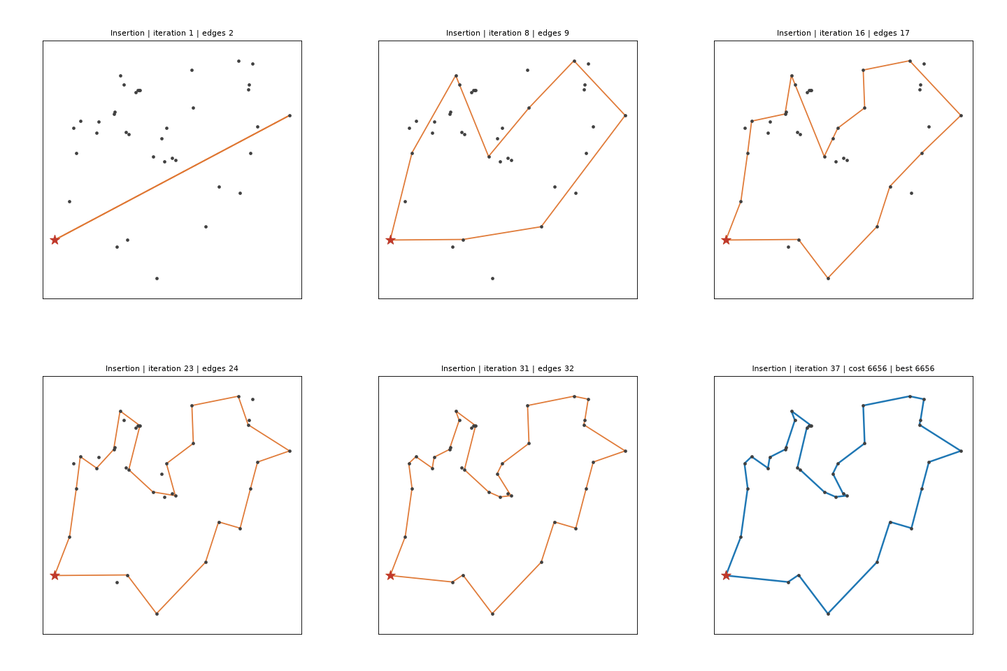
>>> from skroute.base import RouteEvent
>>> labels = dj.labels
>>> partial = [labels[0], labels[7], labels[3]]  # the depot and the first two cities inserted
>>> cycle = list(zip(partial, partial[1:] + partial[:1]))  # the closed partial cycle: three edges
>>> step = RouteEvent("Insertion", "iteration", 2, np.nan, np.nan, None, None, ils.problem_, {"edges": cycle})
>>> ax = plot_route(step)
>>> len(ax.lines), len(ax.lines[0].get_xdata()), ax.get_title()  # one line, x0, x1, nan per edge
(1, 9, 'Insertion | 3 edges')

The GIF is Insertion() (farthest insertion) on dj38, one frame per inserted city — a construction runs in a millisecond, so the file is written at a fixed frame rate rather than as a time-lapse:

python examples/live_demo.py --instance dj38 --solver Insertion --record docs/images/construction_demo.gif --fps 8

Pheromone trails and the SOM ring

Two more extra keys describe structures that are not tours. AntColony reports extra["edge_weights"], floats in [0, 1] parallel to extra["edges"] — the pheromone strength of its 3n strongest trails after each iteration — which LivePlot and Recorder draw under the tours as segments whose width and opacity grow with the weight, so the strong trails stand out and the weak ones fade (Plotly, which cannot vary the width along a trace, draws at one width the trails whose weight reaches a quarter of the strongest one's — MILP's fractional edges included). SOM reports extra["ring"], an (m, 2) array with the positions of its neurons in the units of problem.coords after each epoch, drawn as a closed teal polyline with small markers — the elastic ring closing on the cities while the decoded tour (thin) and the best epoch's tour (thick) follow it:

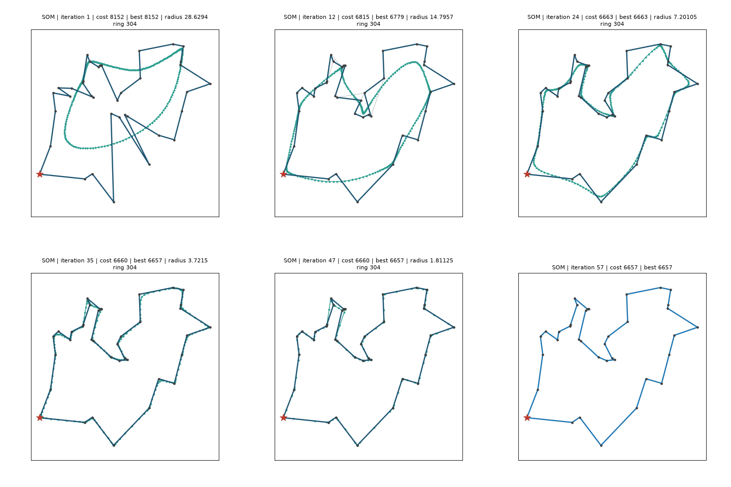
python examples/live_demo.py --instance dj38 --solver SOM --set n_iter=20000 --record docs/images/som_demo.gif --fps 12

Viewers ignore keys they do not know, and an event without a key clears that drawing, so a callback of your own can carry any structure through extra and still be drawn by the three tools when it uses these names. The status line counts them: edges 37, ring 304.

Stop a run interactively

Any callback that returns True asks the solver to stop after its current outer iteration; the fit then completes normally with stop_reason_ == "callback" and the best tour found so far. LivePlot.stop() arms exactly that, for the run in progress (a later fit with the same LivePlot starts unarmed).

Redraws happen on the thread that runs fit, and matplotlib is not thread-safe — the reason MultiStart forwards the callback to its inner estimators only with n_jobs=1. With a desktop window (macosx, Tk, Qt) fit therefore stays on the main thread and the stop comes from the window itself: connect a key handler once the figure exists.

>>> live = LivePlot(dj.coords, every=5)
>>> def watch(event):
...     stop = live(event)
...     if event.stage == "start":  # the figure exists now: any key press stops the run
...         live.fig.canvas.mpl_connect("key_press_event", lambda key_event: live.stop())
...     return stop
>>> sa = SimulatedAnnealing(random_state=0).fit(dj.distance_matrix(), labels=dj.labels, callback=watch)  # doctest: +SKIP
>>> sa.stop_reason_  # doctest: +SKIP
'callback'

In a notebook with %matplotlib inline or backend="plotly" the redraws are IPython.display calls rather than GUI drawing, so the fit can run in a worker thread (the kernel stays responsive) and stop() comes from another cell:

>>> import threading
>>> live = LivePlot(dj.coords, every=5)
>>> sa = SimulatedAnnealing(random_state=0)
>>> worker = threading.Thread(
...     target=sa.fit, args=(dj.distance_matrix(),), kwargs={"labels": dj.labels, "callback": live}
... )
>>> worker.start()  # doctest: +SKIP
>>> live.stop()  # from another cell, a few seconds later  # doctest: +SKIP
>>> worker.join(); sa.stop_reason_  # doctest: +SKIP
'callback'

Maps

The five road-cost tables of skroute.datasets carry (latitude, longitude) coordinates. plot_route_map draws a solution on OpenStreetMap tiles with Plotly's Scattermap, and map=True does the same for LivePlot, Recorder.replay (both then draw with the plotly backend) and Recorder.to_plotly:

>>> from skroute.datasets import load_barcelona
>>> from skroute.viz import plot_route_map
>>> bcn = load_barcelona()  # 19 places, costs in EUR, coords are (lat, lon)
>>> ils = IteratedLocalSearch(random_state=0).fit(bcn.cost, labels=bcn.labels, coords=bcn.coords)
>>> fig = plot_route_map(ils)
>>> [t.type for t in fig.data], fig.layout.map.style
(['scattermap', 'scattermap', 'scattermap'], 'open-street-map')
>>> fig.show()  # doctest: +SKIP
>>> live = LivePlot(bcn.coords, backend="plotly", map=True, every=10)  # doctest: +SKIP
>>> ax = plot_route(ils, bcn.coords[:, ::-1])  # the same route on plain axes: x = longitude

Multi-trip solutions get one Scattermap line per trip. The tiles are fetched by the browser that renders the figure, so a saved HTML file needs a network connection to show the map; the routes themselves are embedded. names= puts a name per node in the hover text — a sequence in matrix row order or a mapping from label to name — and trip_names= names the days and shows them in a legend:

>>> days = IteratedLocalSearch(random_state=0).fit(
...     bcn.cost, labels=bcn.labels, coords=bcn.coords, time_matrix=bcn.time, max_time_work=6.0
... )  # the bundled times are hours: two 6-hour days
>>> places = {label: f"Place {label}" for label in bcn.labels}
>>> fig = plot_route_map(days, names=places, trip_names=["Monday", "Tuesday"])
>>> fig.data[1].text, [t.name for t in fig.data[2:]], fig.layout.showlegend
(('Place 10000007',), ['Monday', 'Tuesday'], True)

Take the plan to Google Maps

A plan is followed on a phone, not in a notebook. skroute.viz.google_maps — no viz extra needed, neither matplotlib nor plotly — exports a fitted solver, a RouteEvent or a plain route (an open tour, a closed one or a multi-trip route with the depot repeated between the days, with coords= as (latitude, longitude) rows and labels= naming them) in three forms that Google Maps understands. Every trip becomes one day, depot → stops → depot, numbered in driving order and coloured from the same ten-colour palette as plot_route_map.

Links. google_maps_urls returns one list of Directions links per day (https://www.google.com/maps/dir/?api=1&origin=...&destination=...&waypoints=...&travelmode=driving, coordinates with six decimals). The Maps URL scheme takes at most nine waypoints between the origin and the destination, so a longer day is split into consecutive legs that share their boundary stop: the first leaves the depot, the last returns to it, and each opens in a browser or in the Google Maps app with turn-by-turn navigation. mode= picks "driving", "walking", "bicycling" or "transit" (Google ignores waypoints in transit mode) and max_waypoints= lowers the limit: Google documents nine waypoints on the desktop site and in the Google Maps app but only three in a phone's browser, so pass max_waypoints=3 for links that will be opened there without the app.

>>> from skroute.viz import google_maps_html, google_maps_urls, to_kml
>>> urls = google_maps_urls(days)
>>> stops = [len(trip) - 2 for trip in days.trips_]  # stops per day; how the solver split them
>>> len(urls) == days.n_trips_ and all(len(day) == (m + 8) // 9 for day, m in zip(urls, stops))  # ceil(m / 9) legs
True
>>> urls[0][0].startswith("https://www.google.com/maps/dir/?api=1&origin=41.398568%2C2.167441&destination=")
True
>>> all(link.endswith("&travelmode=driving") for day in urls for link in day)
True

KML. to_kml writes a KML 2.2 file: the depot as one placemark, one folder per day — named trip_names[k] or "Day k" — holding a placemark per stop ("k.j <name>", described as "Day k, stop j of m") and a LineString of the closed trip, with a line style of its own colour per day (colors=). names= labels the stops, depot_name= the depot. To put it on your phone, open Google My Maps, Create a new map, then in the untitled layer choose Import and pick the .kml — every folder arrives as a group of numbered pins with its line, and the map is available in the Google Maps app under Saved → Maps. Google Earth opens the file directly (File → Open on the desktop, Projects → Open → Import KML file on the web). The KML lines join the stops as the crow flies; the page below draws the roads.

>>> import tempfile, xml.etree.ElementTree as ET
>>> from pathlib import Path
>>> out = Path(tempfile.mkdtemp())
>>> kml = to_kml(days, path=out / "barcelona.kml", names=places, trip_names=["Monday", "Tuesday"])
>>> root = ET.parse(kml).getroot()
>>> ns = {"k": "http://www.opengis.net/kml/2.2"}
>>> folders = list(root.iterfind(".//k:Folder", ns))
>>> [f.findtext("k:name", namespaces=ns) for f in folders]
['Monday', 'Tuesday']
>>> [len(f.findall("k:Placemark", ns)) - 1 for f in folders] == stops  # a pin per stop, plus the line
True
>>> first = folders[0].find("k:Placemark", ns)  # "1.1 Place <label of the first stop>", "Day 1, stop 1 of m"
>>> first.findtext("k:name", namespaces=ns) == f"1.1 {places[days.trips_[0][1]]}", first.findtext("k:description", namespaces=ns) == f"Day 1, stop 1 of {stops[0]}"
(True, True)

A page with the real roads. google_maps_html writes a standalone HTML page that loads the Maps JavaScript API with your key (api_key= or the GOOGLE_MAPS_API_KEY environment variable) and asks a DirectionsService for the roads of every day — one request per leg of at most 25 waypoints, split like the links — drawn by a DirectionsRenderer in the day's colour with numbered markers at the stops and a star at the depot; a legend lists the days with a checkbox each (hide a day, its roads and markers go), the stops and the driving minutes, and a leg whose request fails is drawn as a dashed straight line and reported under the legend (the requests go out two at a time, and one refused for quota is asked once more). The plan is embedded as one JSON object (<script type="application/json" id="skroute-plan">) computed in Python: the stops of each day with their coordinates and names, the legs, the colours, and totals — n_stops and, when the fit had a time matrix, driving_minutes (the matrix is taken to be in minutes, as skroute.preprocessing.travel_time_matrix returns it). The Maps JavaScript API and the Directions requests are billed to the key's project, and the key is written into the page — share the file accordingly.

>>> import json, re
>>> minutes = IteratedLocalSearch(random_state=0).fit(
...     bcn.cost, labels=bcn.labels, coords=bcn.coords, time_matrix=bcn.time * 60, max_time_work=360
... )  # the same two days with the times in minutes, as the page expects
>>> page = google_maps_html(minutes, path=out / "barcelona.html", api_key="AIza-demo", title="Barcelona, two days")
>>> text = page.read_text(encoding="utf-8")
>>> plan = json.loads(re.search(r'id="skroute-plan">(.*?)</script>', text, re.S).group(1))
>>> plan["totals"]["n_trips"] == minutes.n_trips_, plan["totals"]["n_stops"], abs(plan["totals"]["driving_minutes"] - float(minutes.trip_times_.sum())) < 0.1
(True, 18, True)
>>> [(t["name"], t["n_stops"], t["legs"]) for t in plan["trips"]] == [
...     (f"Day {k}", len(trip) - 2, [[0, len(trip) - 1]]) for k, trip in enumerate(minutes.trips_, start=1)
... ]  # one request per day: none has more than 25 stops
True
>>> text.count("AIza-demo")  # the key appears once, in the script URL
1

The key-free interactive alternative stays plot_route_map above: Plotly on OpenStreetMap tiles, with the same names= and trip_names=.

What each solver reports in extra

Every event carries the same core fields — solver, stage, iteration, cost (the objective of the current tour, nan when the solver has none), best_cost, tour and best_tour (label-space open giant tours, depot first), problem, and the decoded route and trips of the best tour — plus extra, a dict of solver-specific facts. The keys of the "iteration" events (each solver's docstring is the reference):

Solver	extra keys	Meaning
SimulatedAnnealing	temperature, accepted, n_moves	the level's temperature, proposals accepted in the level, moves tried ("start" carries temperature = t0_)
TabuSearch	tenure	the tenure applied in the iteration
Genetic	generation, n_evaluations, mean_cost, n_duplicates	generations completed, objective evaluations so far, mean objective of the population, duplicate individuals
AntColony	n_ants, iteration_best, deposit, edges, edge_weights	ants per iteration, the iteration-best ant's cost, whose tour reinforced the trail ("global" or "iteration"); the 3n strongest trails and their strength in [0, 1] (D31)
IteratedLocalSearch	kick, accepted, current_cost	the cut positions of the kicks applied (a list of tuples), whether the candidate replaced the current tour, the current tour's cost
TwoOpt, OrOpt, LocalSearch	moves_applied, gain	the listed moves whose descent changed the tour (a list; "start" carries moves, the ones listed), the iteration's total cost change (<= 0)
SOM	radius, learning_rate, n_samples, ring	neighbourhood radius and learning rate after the epoch's decay, samples presented ("start" also n_units); the neurons' positions after the epoch, (n_units, 2) in the units of coords (D31)
MILP	edges, edge_weights, n_components, lower_bound, objective, n_cuts	the LP support as (label, label) pairs (a list) and the solver's value of each support edge in [0, 1] (D31: drawn as weighted trails), its connected components, the bound, the solve's objective, constraints added so far — one event per cut round
NearestNeighbour, Insertion, ClarkeWright, NRBS	edges (ClarkeWright also n_trips, NRBS also n_edges)	one event per construction step with tour=None and nan costs: the partial path, cycle, trips (and their count) or edge set (and its size) held so far (D31)
MultiStart, EnsembleSimulatedAnnealing, EnsembleGenetic	restart on every forwarded inner event; n_restarts on their own "start"	index of the restart that emitted the event
BruteForce, HeldKarp	—	"start" and "end" only

LivePlot puts one scalar fact — bool, int, float or str: temperature, tenure, mean_cost, generation, iteration_best, radius, lower_bound... the first present in that order of preference, else the first scalar of extra (restart is always shown) — in the title and never lists such as kick and moves_applied; the three structures are drawn instead and counted in the title. The rows are facts of the solvers, not of this page:

>>> def iteration_keys(solver):
...     seen = set()
...     solver.fit(dj.distance_matrix(), labels=dj.labels, callback=lambda e: seen.update(e.extra) if e.stage == "iteration" else None)
...     return sorted(seen)
>>> iteration_keys(IteratedLocalSearch(n_iter=3, patience=None, random_state=0))
['accepted', 'current_cost', 'kick']
>>> iteration_keys(SimulatedAnnealing(random_state=0))
['accepted', 'n_moves', 'temperature']
>>> iteration_keys(TwoOpt())
['gain', 'moves_applied']
>>> from skroute import MILP, NRBS, ClarkeWright
>>> iteration_keys(ClarkeWright()), iteration_keys(NRBS())
(['edges', 'n_trips'], ['edges', 'n_edges'])
>>> iteration_keys(MILP())
['edge_weights', 'edges', 'lower_bound', 'n_components', 'n_cuts', 'objective']

Writing your own callback is the same one-argument function:

>>> def log_improvements(event):
...     if event.stage == "iteration" and event.iteration % 100 == 0:
...         print(event.iteration, round(event.best_cost, 1), event.extra)
...     return False  # True would stop the run
>>> SimulatedAnnealing(random_state=0).fit(dj.distance_matrix(), labels=dj.labels, callback=log_improvements)  # doctest: +SKIP